This is the first in a series of posts about problems, algorithms,
efficiency, how to compare the difficulty of problems, and calling
in on the way to an open problem in mathematics that's literally
worth a million dollars.
But first, let's talk about sums.
Setting the scene with addition
We'll start with some school arithmetic. We learn how to add two
numbers that each have a single digit. What is 3 plus 5? What is
4 plus 9? We learn these single digit sums, and if we forget we
can just add things up on our fingers (and sometimes our toes).
| In case you're wondering, a numeral is a symbol or name
that stands for a number. The number is an idea, the numeral is
how we write it. |
|
But when it comes time to add bigger numbers, we run out of fingers
and toes, and we are forced to use marks on paper. We can use tally
marks, but when you have 643 sheep it's a bit tedious to have to put
a mark for each one. It's better to have the numerals, and then we
want to be able to do arithmetic.
So we learn long addition. (No, I'm not going to talk about long
division!) We learn that we write the two numbers out, one above
the other, and we add them in columns a digit at a time. If the
total for two of these digits in a column is more than 9 then a
"carry" spills over to the next column, and so on.
It's pretty clear that bigger numbers take longer to add, because
there is more to do. Twice the number of digits, twice the time
taken. You might wonder if there would be a faster way to do this,
a question we will return to time and time again, but since we have
to look at every digit it seems reasonable that we can't do better.
We could ask about using binary instead of decimal, or base 8, or
base 60 (as the Babylonians did), and in fact if you've remembered
all of your base 60 single digit sums, then because the numbers are
shorter in base 60 it will take less time. But it's still the case
that twice the digits will take twice the time.
|
Detail: The exact time taken depends on the number of carries.
To take that into account we always talk about worst case
timings, and the timings are considered to be "upper bounds."
A brief note about notation - I will sometimes use a "centre dot"
to represent multiplication, as I have done here, sometimes use a
"lower dot," sometimes use a "times" sign, and sometimes not have
any symbol at all, using juxtaposition. It should, in each case,
be unambiguous that I'm performing a multiplication, and my choice
will largely be driven by aesthetics, although occasionally the
need for clarity and explicitness will override that. However,
if you feel strongly enough about this I invite you to email me
to discuss it. |
|
Similarly, if we do it in binary each column will be quicker, but on
average writing a number in binary takes 3 and a bit times as many
digits as it does in base 10, so it will take three and a bit times
as long to add up. But it's still that case that twice the digits
will take twice the time.
So the time taken to perform the addition is some constant times
the number of digits. The constant will be different for different
bases, etc, but it will still be:
$T=c{\cdot}S$
where $T$ is the time taken, and $S$ is the size (number of digits)
of the numbers involved.
The time taken is linear in the size of the input number(s).
Moving up to multiplication
Now let's have a look at long multiplication. Here's an example:
._______________3___6___5
._______________8___7___2
.______________=========== \
._______________6__12__10___\___Central
.__________21__42__35________>__Section
.______24__48__40___________/
._____==================== /
.______24__69__88__47__10
.
.______31___8___2___8___0
I've done this is a slightly unusual way to emphasise that the central
section of the table is made up of the products of the individual digits
of the initial numbers. The final number is made up by adding columns
and carrying digits as necessary.
We can ask how long this will take. Well, if we have $n$ digits in the
first number, and $m$ digits in the second number, we have $nm$ products
in the central section. Then we have up to $m$ rows to add, each with
$n$ numbers, but they are skewed, so we have $n+m-1$ columns in total.
The exact time taken for two specific numbers will depend on the number
of carries we have to perform, but careful analysis (which we won't do
here) shows that there are constants $c_2,$ $c_1,$ and $c_0$ such that
when $k$ is the number of digits in the larger number, the time taken,
$T(k),$ will be given by (or at least will be bounded by):
$T(k)=c_2.k^2+c_1.k+c_0$
That sounds complicated.
But this is where a simplification comes to our rescue - we choose to
ignore the constants involved and just look at the general shape of the
function. In short, the time taken to multiply will be dictated by
the number of cells we have to complete in the above table, and that's
proportional to $mn.$ As the numbers to be multiplied get larger and
larger, so the time taken gets totally dominated by the first term,
$c_2k^2,$ so we ignore the exact value of the constant $c_2$ and say
that this algorithm is $k^2$ in the size of the input numbers.
It's quadratic.
So, in summary, the time taken by this algorithm is quadratic because
for two numbers - say they're both the same length - the number of cells
in the middle is quadratic, and that's the bulk of the work as numbers
get bigger.
Is there a better way?
When we multiply, clearly we have to look at each digit at least once,
so it's certainly true that we can't multiply numbers in better than
time that's linear in the size (in digits) of the numbers involved.
We've seen here that the usual school algorithm is quadratic, so the
question is: can we do better?
As it happens, yes we can. There are algorithms that are significantly
faster, but for smaller numbers the extra house-keeping is horrendous
and absolutely not worth it. However there are contexts where we are
dealing with very, very large numbers - cryptography is one example
- and in those cases it really can make a difference. So there are
algorithms that are much faster for multiplying really, really large
numbers. We'll mention one later.
| In this section we start to look at how we might compare the
difficulty of two problems. Is problem $A$ harder than problem $B$?
Or is it easier? How can we tell? What does it mean? Here we start
to answer those questions. |
|
Squaring is easier than General Multiplication. Or is it?
We've been looking at general multiplication, but we might wonder if
it's easier in the special case of the two numbers being equal. It's
obvious that if we can do general multiplication then we can square,
but what if we can square things quickly.
| The oracle is a device we use to think about the comparative
difficulty of problems. As a thought experiment we say: "What if we
could solve problem $P$ instantly - what would that then allow us to
do with a small amount or extra work?" The way we express this is to
say: "Let's suppose we have an oracle to do this complicated thing -
what can we do then?"
So here we are saying: "Let's assume we can square numbers instantly
and for free. What would the consequences be of that?" The answer
is that with a little extra work (which takes linear time) we could
then perform arbitrary multiplications. Which is kinda cool.
Later we will return to the oracle idea and use it in a much more
difficult/complicated setting.
|
|
What if we had an oracle to square numbers instantly? Could we use
the oracle somehow to multiply any two numbers?
The answer is, perhaps surprising, yes, we can. Here's how.
Start with two numbers, $a$ and $b.$ As an example I'll use 256 and
139, but I suggest you pick your own and play along.
We compute their sum, $s=a+b,$ which in my case is $395.$ We also
compute their difference, $d=a-b,$ which in my example is $117.$
The numbers $s$ and $d$ are then sent to our oracle which instantly
calculates $s^2$ and $d^2,$ which in my case are $s^2=156025$ and
$d^2=13689.$ And now the small piece of magic is that the product
$ab$ is the difference between $s^2$ and $d^2,$ all divided by 4. So
in this case you can check that $256{\times}139$ is $(s**2-d**2)/4,$
which is $(156025-13689)/4,$ which is 35584.
| Exactly how this works is a useful exercise in elementary
algebra. |
|
And it is.
You should try it with your own numbers just to be sure.
|
You may find this all faintly ridiculous. But this is a single, simple,
concrete example to set up the ideas we'll explore in later articles
where the problems we're trying to solve are unfamiliar, much harder,
currently unsolved, and of immediate use in the "real world." |
|
So that means that if we have a squaring oracle we can, with just some
extra addition, subtraction, and halving, all of which take a linear
amount of time, work out any product we want to. So in some sense we
don't have to know how to do general multiplication, we can just learn
how to square, and then use the above technique. The total time taken
will then be the time the oracle takes, plus the time for our extra
work.
Faster Squaring (and hence faster Multiplication)
Now we can see one method for faster squaring. We can square
numbers with $k$ digits in time faster than $k^2$ as follows.
As an example, let's compute $27182^2.$ We split $27182$ into
$27000+182\;=\;27\times{10^3}+182$ and then compute:
- $27^2=729,$
- $2{\times}27{\times}182\;=\;9828,$
- $182^2=33124.$
Then our result is:
- $729000000+9828000+33124\;=\;738861124.$
|
|
Suppose a number $N$ has $k$ digits, and split $N$ into two pieces,
taking $b$ to be the rightmost half of the digits ( or slightly more
if there are an odd number of digits) and $a$ being the "top half" of
the number, so $N=a{\times}10^h+b$ where $h=k/2$ (rounded up if $k$
is odd). Then we can compute:
$\begin{align}N^2&=(a.10^h+b)(a.10^h+b)\\&={a^2}10^{2h}+2ab10^h+b^2\end{align}$
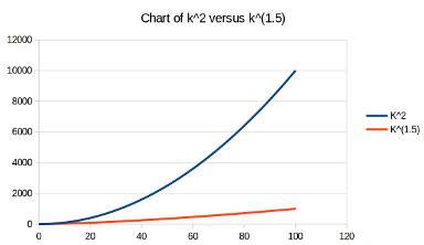
Comparison of $k^2$ versus $k^{1.585}$ |
|
So this shows that we can accomplish the squaring of a $k$ digit number
with two squarings, one multiplication, a doubling, and some additions.
In each case the numbers we are using, $a$ and $b,$ are half the size of
the original ($N$). We convert the multiplication of $a$ and $b$ into a
squaring process, and then repeat the entire process with these smaller
number, $a$ and $b.$ Eventually we get down to single digits, which we
assume we can square or multiply in constant time.
| Proving the time taken to be $k^{log_2(3)}$ is beyond the scope of
this article, but broadly speaking it goes like this. Let $T(k)$ be
the time taken either to square a $k$ digit number or to multiply two
$k$ digit numbers. Then $T(k)\;=\;3T(k/2)$ plus linear terms. We can
verify that $T(k)\;=\;k^{log_2(3)}$ satisfies that relationship. |
|
Analysing this shows that the time taken to square a number is now
proportional to $k^{log_2(3)},$ and $log_2(3)$ is about $1.585$ or so.
This power is much smaller than 2, so the time taken grows
much more
slowly than $k^2.$ The cost is all the extra fiddling about and
remembering intermediate results.
But if the numbers are huge to start with, this is definitely worth it.
We can now use this to create a faster algorithm for multiplication via
squaring. Alternatively, by using this as our inspiration it's also
possible to find a similarly convoluted algorithm for multiplication
that also runs in time proportional to $k^{1.585}.$
To see how, suppose we want to multiply $a$ and $b,$ and suppose they
have $k$ decimal digits. As before, let $h$ be $k/2$ rounded up, and
write $a$ and $b$ as $a_1s+a_0$ and $b_1s+b_0,$ where $s=10^h.$ In
essence, we write each of $a$ and $b$ as a combination of their upper
and lower halves (digit-wise).
| Where these particular sums and products come from is the magic
in this method, and is down to the inventive genius of the people who
first came up with the technique. You are expected neither to come up
with this yourself, nor to see immediately where they come from. To
say that sort of thing always feels a little unsatisfactory, but it's
one of those tricks that you learn as a trick, and which then becomes
more obvious and "natural" as you become more familiar with the area.
|
|
If we write $u=a_1b_1$ and $l=a_0b_0$ (for upper and lower products)
and we write $d=(a_1+a_0)(b_1+b_0)-(u+l)$ (although at first glance
there is no obvious reason why we should do this) then we find that:
$ab=us^2+ds+l$
Thus we have accomplished a general multiplication with three smaller
multiply operations and some linear operations. Verifying the details
is left to the (possibly mythical) interested reader.
Clarifying the words we use
So we've talked about Squaring and Multiplying - we think of these as
problems to solve, and the algorithms we use are the solutions. But
what exactly do we mean by "a problem"?
In the case of squaring (which we've seen is, with a little extra work,
the same as multiplying) we have an infinite collection of numbers, and
for each number we ask the question: What is its square?
Loosely speaking we can say that:
- The problem of SQR is ...
- a collection of numbers of which ...
- we ask "What is the square"?
| An algorithm is a set of rules and/or processes to follow,
which can be given an input, is guaranteed to terminate, and produces
an output.
|
|
A
solution to the problem of
SQR is an
algorithm which, when given
a particular number, will return the square of that number.
Now let's generalise.
- A problem is ...
- a collection of things (which we call "questions" or "instances") ...
- each of which has an associated other thing (which we call the "answer" or "result") ...
- which we want returned to us when we "ask the question".
Sometimes a given question will have a collection of answers, any one
of which will do. In the case of "Factoring" (which we talk about
shortly) a "Question" is a positive
integer of which we want a factor,
and the "answer" is simply any non-trivial factor. Some formulations
of the factoring problem require
all factors to be returned, but that
is a detail we need not consider (yet).
|
We talk about the "Time Complexity" of an algorithm, being the function
that gives us an upper bound for the worst case performance of that
algorithm. When we talk about the time complexity of a problem we
mean the time complexity of the best possible algorithm. Of course,
sometimes we don't know the best possible algorithm, sometimes we only
know the best algorithm so far. That being the case, we talk about
the currently known time complexity of an algorithm, although we often
just say "the complexity" and assume the listener/reader knows that we
mean the "currently best known time complexity."
Specifically, it is still an open challenge in computing as to what the
best possible algorithm is for multiplication.
|
|
So:
- The "things" in the collection are called instances or questions,
- The things we get back are called answers, results, or responses.
- A solution to a problem is an algorithm which ...
- when given an instance ...
- returns to us the associated result.
In the specific example of the problem
SQR we have:
- The instances of the problem SQR are numbers,
- The results are the squares of those numbers, and
- We have two solutions, two algorithms, which are given above.
Summarising, and at the risk of repeating ourselves somewhat, we take
the technical definitions to be that:
- A Problem is a collection of things about which we ask a specific question.
- We call these things instances.
- Each instance has an associated answer or result.
- A Solution for a problem is an algorithm that when given an instance will give back the desired response.
- The Time Complexity of an algorithm is the function that tells us, as a worst case, how long it will take to find the result for a given question.
- We usually just ask for the dominating form of the function.
|
When we compute how long an algorithm takes in the worst case we are
usually only concerned about the behaviour in the long run, as the
inputs get larger and larger. As such, if the time complexity of an
algorithm is something like $a_2x^2+a_1x+a_0,$ we don't much care
about the $x$ term or the constant term, because in the long run they
will be overwhelmed by the $a_2x^2$ term. That's what we mean by the
"dominating form" of the function.
|
|
So we can talk about the "problem of squaring" as being the (infinite)
collection of numbers to be squared. As we have seen above, the time
complexity of addition is linear, the
time complexity of multiplication
is at worst quadratic (although it's actually at worst $k^{1.585},$ and
in fact it's the subject of on-going research, and is now known to be
better than that), and the
time complexity of squaring is effectively
the same as that for multiplication.
Finally, the time complexity is, after all, a function, and so far I've
talked about it being of an algorithm. So the function needs an input.
What is the input?
| Technical point: The notation $O(...)$ is used to denote the
upper bound of the time complexity of an algorithm. We then abuse the
notation to use it to refer to the time complexity of the best known
algorithm for a problem. Using this notation:
$O(MUL)\;=\;O(SQR)$ |
|
What we are interested in is how long the algorithm takes as a
function
of the
size of the instance it's given. Multiplying numbers takes
more and more time as the numbers get bigger. The
time complexity is
a
function of the
size of the instances. So for the algorithm for
squaring, the
time complexity is $M(s)$ where $s$ is the size of the
instance. But what is the size of the instance?
The size of the instance is the number of bits required to specify it.
This amounts to saying - it's the number of symbols required to write
it down.
On this basis, 123456 is twice the size (as an instance) as 123, and
that matches how we deal with it when we multiply by it or square it.
It's the number of symbols involved that dictates the amount of work
we have to do - and that feels like a reasonable definition.
The inverse of Multiplication - the problem of Factoring
| Technical point:
For some problems we just want a Yes/No result, but for others we want
some sort of object. In the case of multiplication we want to know what
the product is, in the case of factoring we want to know an specific
factor, but for other problems we just want to know "Is this possible"?
The latter type of problem is called a "Decision Problem" and they turn
out to be critically important. However, it is often the case that an
algorithm for a decision problem can be converted into an algorithm to
give us an actual result. We will return to this later. |
|
Let's look at another problem:
Factoring integers. For this problem we
are given an
integer and we are asked to find a
divisor - also called a
"factor." There is a simple algorithm to do this: Start at 2 and see if
that's a
divisor. If it is, stop, otherwise ask about 3, then 4, then 5,
and so on. This process must eventually stop, because every number is
divisible by itself. When it does stop, it will have found a (possibly
trivial)
divisor.
The problem with this algorithm is that it's slow. Really slow. If you
have a five decimal digit number then you might have to perform tens of
thousands of trial divisions. Indeed, if the number you're given is
prime then you will have to try every number up to that.
| In symbols, if $N$ is not prime then there exists $f$ such that
$1<f\le\sqrt{N}$ and $f|N.$ |
|
Of course we can improve this enormously. For one thing, if there
is
a non-trivial factor then there must be at least one factor that is no
more than $\sqrt{N},$ where $N$ is the number we are trying to factor.
That means we can abort the process as soon as we get to $\sqrt{N}.$
If we haven't found a factor by then, then $N$ is prime.
|
It's a real drag to keep saying "non-trivial factor," so from now on
we'll assume that we're talking about non-trivial factors unless the
the context clearly requires otherwise, or unless explicitly stated.
|
|
As a further refinement, if $N$ isn't divisible by 2 then it won't be
divisible by any even number, so we don't have to bother dividing by 4,
6, 8, and so on. Taking that argument to its logical conclusion, we
only need to test primes as potential
divisors.
How does all that help? If $N$ has $k$ decimal digits then the initial
algorithm potentially has us trial dividing by up to some $10^k$ times.
The first refinement means we only need to trial divide by numbers up
to $\sqrt{N}$. That's about half the number of digits, and so is about
$10^{(k/2)}.$
To see what effect the second refinement has, where we only divide by
primes, we need to know how many primes there are up to a given number.
The first major results about this were by Gauss and Legendre, who
showed that the number of primes up to $m$ is around $m\frac{1}{ln(m)}.$
For a number with $k$ decimal digits, the square root will be about
$10^{k/2},$ so we can work out that the number of divisions needed is
roughly, very roughly, about $\frac{1}{k}\times(10)^{k/2}.$ That's
a bit more than $\frac{1}{k}\times{3}^k.$ (It's worth noting that $3^k$
grows so fast, dividing by $k$ really makes next to no difference.)
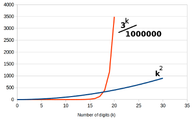
Comparison of $k^2$ versus $3^k$ |
|
Even so, for a number with $k$ digits, we may still need to perform
an exponential number of trial divisions - $b^k$ where $b$ is some
constant. The
time complexity of this algorithm for factoring is not
polynomial in the size of the instance, it is exponential. The chart
here at right shows just how catastrophic that is. Here we have
charted $k^2$ against one millionth of $3^k.$ We are imagining that
the trial divisions run a million times faster than anything else, and
while that helps for a while, it doesn't take long for the exponential
nature of $3^k$ to take over, and the time taken just explodes.
And in truth it's worse than that, because as the numbers get larger
the individual divisions take longer and longer. Even so, the effect
is completely swamped by the exponential number of divisions required.
It's interesting to note that the operation of factoring is effectively
an inverse to the operation of multiplication. So we have two problems
that are inverses of each other, and yet MUL is relatively easy, while
FAC is apparently difficult.
And I say "apparently" here because in truth
we just don't know how bad factoring really is.
There are some phenomenally clever algorithms now, much cleverer than
simple trial division, that take time that is less than exponential, but
more than polynomial. That's a little hard to take in, and the exact
circumstances and expressions are tricky, but so far, with our current
theoretical understanding, and using classical (non-quantum) computers,
the time complexity of integer factoring is super-polynomial, but
sub-exponential.
We need to remember here that when we talk about the time complexity of
an algorithm we are talking about the worst case. Most random numbers
that you pick can be factored quite quickly - the proportion of numbers
that are actually difficult to factor is quite small, and gets smaller
as you deal with larger and larger numbers. After all, if you pick a
large random number there's a 50% chance it will be even, making it
trivial to find a factor. Even if it's odd there's a 33% chance it will
have 3 as a factor. And so on. So in a very real sense, most numbers
are "easy to factor."
But some are hard (with our current understanding), and those are the
ones we have to worry about when we discuss the time complexity of an
algorithm.
Pause for a summary so far ...
- A Problem is a collection of questions - we call them instances
- An Algorithm is a recipe for taking an instance and finding the (or an) result
- We can talk about the time the algorithm will take
- ... which is a function of the size of the question
- Addition has linear time complexity
- Multiplication has at worst quadratic time complexity
- ... but in fact there are faster algorithms
- If we can have an algorithm to square then we can do a bit of extra work and create an algorithm to multiply
- Integer factoring has no known polynomial algorithm,
- but it does have algorithms that are faster than exponential.
- Most integers are easy to factor,
- ... but time complexity is an upper bound for all cases
- ... and therefore we worry about the worst case questions.
Factoring versus Multiplication
So we have a clear connection between factorisation and multiplication.
We multiply $5$ by $7$ to get $35,$ we take $35$ and factor it into $5$
and $7.$ Because of this we can think of MUL and FAC as inverse
problems, and we might wonder if somehow we can use one to solve the
other. In other words, suppose we have an algorithm to multiply two
numbers really, really quickly. What we want to know is whether we can
use that to create an algorithm to factor quickly.
| You may notice that although we have assumed that we have an
algorithm to multiply, and we are trying to derive an algorithm based
on that to get an algorithm for factoring, the algorithm described here
does not, in fact, use multiplication. It uses division.
However, just as we can take an algorithm for squaring and use it to
create an algorithm for general multiplication, so we can take an
algorithm for multiplication and with a bit of extra work use it to
create an algorithm for division. I'm not going to do that here, you
could regard it as an exercise for the interested reader. |
|
Let's suppose we want to factor $N.$ Consider the following algorithm:
- Pick a possible factor, call it $F.$
- Attempt to divide $F$ into $N.$
- If there is no remainder, we're done.
- Otherwise go back to the beginning and pick another number.
Of course, our chosen possible factor $F$ has only a miniscule chance
of actually being a factor, but we observe that each loop through this
process only takes a
polynomial amount of time. The trouble is that in
general we will have to make a lot of guesses to make it work! A quick
check shows that "on average" we will need to make just as many guesses
in this process as we did in the trial division algorithm we looked at
earlier. In that sense this algorithm is no better than the trial
division algorithm, but we will soon see what we have gained by thinking
about it this way.
Emergence of the definition of $\mathcal{NP}$ ...
What we've described in the previous section is what we call a
"non-deterministic" algorithm - one that has guessing as an integral
part of the algorithm. Since for each guess the algorithm takes a
polynomial amount of time, so we call this a "non-deterministic
polynomial time algorithm." The general idea is that it's quick,
provided we guess right.
| We use the $\mathcal{script}$ font because we are going up a
level, so to speak. The sets $\mathcal{P}$ and $\mathcal{NP}$ are
sets of problems, and problems are themselves sets of instances. It's
useful to be able to call a problem $P$ so it's useful to have a
different font for sets of problems. In this case, $\mathcal{P}$ and
$\mathcal{NP}$ are very specific sets of problems.
The term "non-deterministic" is, perhaps unsurprisingly, the
complement of the term "deterministic." It refers to the idea that
the outcome is not rigidly determined, but instead that randomness or
guesses are somehow involved. |
|
This turns out to be a useful concept, so we give it a special name.
Consider all problems that have a non-deterministic
polynomial time
algorithm to solve them.
We call the set of all such problems $\mathcal{NP}.$
We have seen about that
FAC has a non-deterministic
polynomial time
algorithm, so the problem
FAC is in the set $\mathcal{NP}.$ Thus
FAC is called an $\mathcal{NP}$ problem.
So just to recap, an $\mathcal{NP}$ problem is one that has an algorithm
like this:
- Pick a candidate result
- taking no more than polynomial time to make the selection
- and which might simply be a guess
- Check it using a polynomial time algorithm
- If it works, report success and stop
- If not, go back to step one.
So we can see that the problem
FAC (
Integer Factorisation) falls into
this category. We can just guess a possible factor and then divide or
multiply to see if it is right. So
FAC is in $\mathcal{NP},$ it is
an $\mathcal{NP}$ problem.
This sounds stupid, but it's important
Warning: This section is quite tricky, and some care is required.
Do not expect to read this section "like a novel" - it will take
time and thought. It's a challenge, but is an excellent warm-up
and preparation for the pay-off that comes later.
| The set of all problems that can be solved in polynomial time
is written $\mathcal{P},$ and such problems are referred to as
"polynomial problems." This does not mean that the problems relate
to polynomials, it means that there is an algorithm that takes an
instance and returns an appropriate result, and that algorithm takes
polynomial time. |
|
Let's consider a problem that can be solved in
polynomial time - let's
call it $P.$. Remember, a
problem is a collection of questions. So
$P$ is a
polynomial problem, which is to say that we have an algorithm
$\mathcal{A}$ that given an instance from $P$ can return a result in
polynomial time.
And we ask:
- Is problem $P$ in the class of problems $\mathcal{NP}$ ?
That's a good question, and the answer is yes. How do we show that?
We simply use the definitions we're given.
How?
We want to show that $P$ is in $\mathcal{NP}.$ By definition, that
means we need to demonstrate that we can follow this process:
| Note here we are using the alternate term "question" instead
of "instance." |
|
- Given a question $Q$ in problem $P:$
- Guess a candidate result $R$
- Check the candidate in polynomial time
What do we know? We know that $P$ is a
polynomial time problem, and
that means there is an algorithm $\mathcal{A}$ which given a question
$Q$ in problem $P$ will compute the result $R$ in
polynomial time.
|
After we've guessed a candidate result we need to check whether or
not it is, in fact, correct. But the only thing we know about $P$
is that there exists algorithm $\mathcal{A}$ which will give us the
appropriate $R.$ So quite literally the only thing we can do is
compute the actual result and then see if they are the same.
And I know that it seems stupid that we would repeatedly compute
$\mathcal{A}(Q)$ - the point is that we must show that $P$ is of
this form. That doesn't mean this is what we would do in practice!
We're doing this purely for the purpose of proving something about
every problem in $\mathcal{P}.$
I refer you to the title of this section. |
|
Here's what we do.
- Guess a candidate $R_0$
- Compute $R_1=\mathcal{A}(Q)$
- This takes polynomial time
- This is how we will check to see if $R_0$ is actually a solution.
- See if $R_0=R_1$
- This takes linear time
- (Not necessarily instantly obvious, but to see if two things are the same we compare them, and that should take no longer than time proportional to the sizes of the objects).
This shows that we can, in fact, follow the procedure that defines
what it means to be $\mathcal{NP},$ and thus the problem $P$ is an
$\mathcal{NP}$ problem.
At this point you might be worried by this whole "Guess a solution"
bit, saying - well, just compute it! Indeed, we can get $R_0$ just
by computing the result, because by assumption we know how to do that.
But to show problem $P$ is in $\mathcal{NP}$ we have to show it's of
the right form.
And we have.
So we have shown that every problem that has a polynomial time algorithm
is in $\mathcal{NP}.$ Remembering that the collection of all problems
that can be solved in polynomial time is called $\mathcal{P},$ what we
have shown is that everything in $\mathcal{P}$ is in $\mathcal{NP}.$ In
other words (well, in symbols, really) we have shown that
$\mathcal{P}\subset\mathcal{NP}.$
The title of this section claims that it's important. Why?
What we have done is to define two entire classes of problems, and then
reason carefully to show that one class is contained entirely inside
the other. This careful reasoning is an example of what we will be
doing later when we define another, very important class, and ask what
relationship it has to these. This section has been a warm up for what
is to come.
Comparing the difficulty of problems
Let's go back to the problems of "Multiplication" and "Squaring". It's
pretty clear that if we have an algorithm to multiply two numbers then
ipso facto we have an algorithm that can square a number. What's less
obvious, but as we saw earlier is in fact true, is that if we have an
algorithm to square a number then we can soup it up into an algorithm
to multiply two numbers. That then means that if we can find a faster
algorithm for SQR then we can use that to create a faster algorithm
for MUL, and vice versa.
So in a very real sense these are "the same problem." The fact that
we can inter-convert them taking no more than linear extra time is
what we mean when we say that neither is significantly more difficult
than the other.
| We are about to compare the difficulty of problems. In doing so
we must reason about algorithms that have not yet been devised, and
which might not actually exist. Traditionally we couch such reasoning
in the form of questions to an oracle. |
|
Now consider two problems, $A$ and $B,$ and let's suppose that someone
else, Olivia the Oracle, has a secret technique for solving $A.$ Using
that, here's a possible technique for solving $B:$
- Take an instance $Q_B$ from $B$
- Convert it into an instance $Q_A$ of $A$
- Let Olivia find the result $R_A$ for $Q_A$
- Convert $R_A$ back into the desired result $R_B$
Of course, this would only be of use if the total time taken for the
conversions plus the the time Olivia takes is smaller than the time
taken to solve $B$ directly, but even so, this is an idea of how we
might be able to parley up Olivia's solution for $A$ into a solution
for $B.$
So the big idea is this. Suppose we can create efficient conversions
of $Q_B$ into $Q_A,$ and $R_A$ into $R_B,$ then any algorithm for $A$
automatically gives us a comparably efficient solution to $B.$ In this
way we can say that if such conversions exist, then problem $A$ is in
a very real sense harder than (or at least as hard as) $B$.
In summary
We've shown that if we can square numbers, then with a little more work
we can multiply numbers in general. In fact, if we have someone who can
magically square numbers for us then with just the extra ability to add,
subtract, and divide by a constant we then have the ability to multiply.
In particular, we now have the ideas of how to compare the difficulty
of different problems, and how to use a solution to one problem to give
us a way to solve another. In short, we are now ready to talk about
Next post:
- What are some problems in NP but not known to be in P?
- How do they compare with FAC?
- How do they compare with each other?
- What is "NP-Complete"?
- Why do we care?
Many thanks to
@RealityMinus3/E.A.Williams and others for detailed
feedback, which has improved this page enormously.
Local neighbourhood - D3